- Information by Map Unit
- Information by Topic
- Documents in SoLo
Links to other related sites
- About SoLo
-
- Mission
- Disclaimer
- Authors (complete list)
The vegetation of "western-montane" forests is outlined in the context of different climatic regimes that vary from inland maritime to continental. Soil/vegetation correlations are most evident in the more severe environments, particularly with granitic versus limestone substrates. In moderate environments, soil/vegetation correlations can be derived but with greater difficulty. In most cases, these correlations are strongest on a local basis; regional correlations are difficult to achieve. Weak soil/vegetation correlations often result from the way soils and plant communities are described and from the effect of compensating factors within plant communities. The problem of compensating factors is illustrated in three soil/vegetation studies. An ecological perspective toward correlating soils and vegetation is emphasized. Combining ecosystem classification with landtype mapping is considered a useful result of the ecological perspective.
Plant communities of western-montane forests vary geographically and largely as a function of climate, topographic influences, and substrate. Site history is also involved. Western-montane forests experience two distinct climatic influences, a Pacific maritime climate occurring mostly during winter and a continental climate during the summer. The relative proportions of these two climatic influences vary geographically: the northernmost areas are predominately maritime and the southeasternmost areas predominately continental. Throughout this broad area, most western-montane forests fall within the Engelmann spruce (Picea engelmannii), western hemlock (Tsuga heterophylla), Douglas-fir (Pseudotsuga menziesii), and ponderosa pine (Pinus ponderosa) floristic provinces of Daubenmire (1978) and the Columbia, Sierran, and Rocky Mountain forest provinces of Bailey (1980).
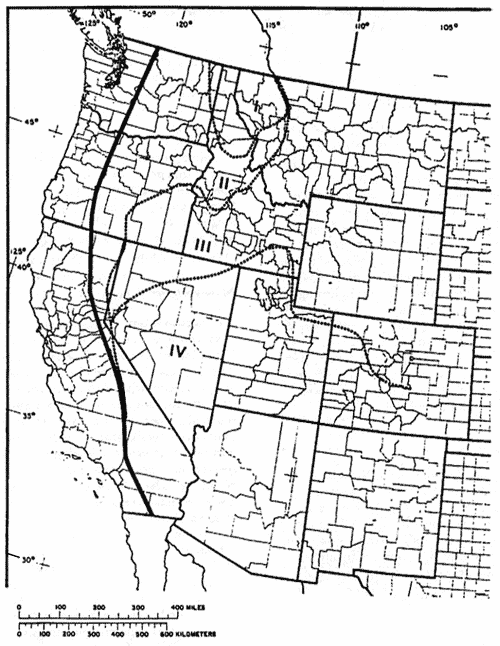
The Pacific maritime influence is most evident in northeastern Washington, northern Idaho, and northwestern Montana. It occurs in diminished and varied forms across much of eastern Washington and Oregon, in west-central Idaho, and along the east slope of the Cascades and Sierra Nevada mountains (fig. 1) in eastern California. These high-mountain ranges intercept much of the maritime moisture and create a rainshadow to the east that precludes forest growth over a vast area.
The moist Pacific air masses are carried inland by the prevailing westerlies and have a dominating influence on vegetation over much of the northern western-montane area (Daubenmire 1969). Extended periods of cloud cover and fog with prolonged cyclonic storms characterize the weather pattern from fall through late spring. During summer, the westerlies shift northward and a weak continental climate creates drought with few clouds during the latter part of the growing season.
The resulting environment is relatively mild in these forests, supporting many plant species that occur largely west of the Cascade-Sierran axis. Western hemlock, western redcedar (Thuja plicata), mountain hemlock (Tsuga mertensiana), western white pine (Pinus monticola), and Pacific yew (Taxus brevifolia) comprise much of the forest found in the core area of maritime influence (fig. 1). Beyond the core area these species decline; this provides greater opportunity for other maritime-dependent species such as western larch (Larix occidentalis) and grand fir (Abies grandis). On the east slope of the Sierras, Jeffrey pine (Pinus jeffreyi) and white fir (Abies concolor var. lowiana) occupy similar conditions. Even ponderosa pine, which occupies the driest forest sites throughout the area, is the variety ponderosa that has Pacific maritime affinities (Steele 1988). In Oregon (Franklin and Dyrness 1973), Idaho, Montana (Arno 1979), and possibly elsewhere, this pine's southern and eastern geographic limits approximate the extent of Pacific maritime flora.
Figure 1—Approximate climatic regions in western-montane forests as suggested by distributions of indicative tree species. (I—core maritime, II—inland maritime, III—northern continental, IV—southern continental). [Text description of this map]
Widespread soil/vegetation correlations may be more difficult to obtain in this inland maritime environment, than in harsher environments that are more restrictive to plant distribution. Much of this area, especially in Idaho and northern Washington, also contains weakly developed forest soils such as those of granitic and aeolian (ashcap) origin as well as skeletal soils of several other rock types. The way soils and plant species have been classified can also lead to poor soil/vegetation relationships. A plant's ability to exploit compensating factors exacerbates these often poor correlations. Some major tree species such as grand fir (Daniels 1969) and Douglas-fir (Rehfeldt 1989) have a broad range of genetic diversity, and other plant species may also be genetically diverse, which may confound soil/vegetation relationships. Consequently, one should not always expect soil/vegetation correlations of inland maritime forests to be easily derived.
In central Idaho, for example, a Douglas-fir/ninebark (Pseudotsuga menziesii/Physocarpus malvaceus) association on basaltic soils is nearly identical to that on granitic soils. Grand fir associations are also similar across these two contrasting parent materials (Steele and others 1981). But toward the environmental extremes of the forest zone such as at lower timberline, soil-controlled differences in vegetation become more evident. For example, a ponderosa pine/bluebunch wheatgrass (Pinus ponderosa/Agropyron spicatum) association, particularly the forb component (Steele and others 1981), on basaltic soils is often different floristically from its counterpart on granitic soils.
On a local basis, some correlations have been derived. Neiman (1986) was able to identify differentiating soil characteristics in several highly similar grand fir and western redcedar associations. In the Garnet Mountains of west-central Montana, limestone and granitic substrates support notably different forest communities (Goldin and Nimlos 1977). Other relationships may emerge as we explore soil/vegetation relationships in more detail.
To the south and east of the inland maritime region lies an area having a stronger continental climatic influence, although the maritime influence remains evident during winter and spring in varying degrees (Bradley 1976). Here summer thunderstorms deliver moisture in downpours during July and August and, in some areas, into September. This moisture moves inland in the form of high-altitude air masses from the Gulf of Mexico and southern California coast resulting in convectional storms over the mountainous areas. Precipitation diminishes as these air masses move inland with only "dry lightning" often available to the inland maritime area of Idaho and western Montana. Rarely is there enough cloud cover to moderate the temperature for a significant period. The vegetation in general is quite different; most forest species of the inland maritime area are absent. Even the forest zone is more restricted, having been replaced at lower elevations by pygmy woodlands and chaparral.
In extreme southeastern Idaho, most of Nevada, Utah (except the Uinta Mountains), southern and western Colorado, Arizona, and New Mexico (fig. 1) there is a somewhat different mix of tree species than is found to the north. These forests are generally found above extensive woodlands of various pinyon, juniper, manzanita, and oak species. In some areas the interior variety of ponderosa pine (Pinus ponderosa var. scopulorum) forms extensive lower timberline forests, often with grass-dominated undergrowths (Hanks and others 1983). But in much of the area, adequate precipitation occurs only at elevations too cold for the pine seedlings to survive. Here Douglas-fir or quaking aspen (Populus tremuloides) usually forms lower timberline, although in some areas mixtures with limber pine (Pinus flexilis) or blue spruce (Picea pungens) may occur. The blue spruce also dominates certain topoedaphic situations such as alluvial or colluvial deposits, frost pockets, and riparian zones. With increasing elevation, and presumably more moisture, a few additional tree species become major forest components. Concolor fir (Abies concolor var. concolor) mixes with the Douglas-fir to form an extensive mid-elevation zone. In Arizona south of the Mogollon Rim, and in southwestern New Mexico, several pines (Pinus strobiformis, P. leiophylla, P. arizonica, P. engelmannii) and associated evergreen oaks (Quercus hypoleucoides, Q. rugosa, Q. arizonica, Q. emoryi) add diversity to these mid- and lower elevation forests (Bassett and others 1987; Layser and Schubert 1979). Many of these species represent a northern extension of Mexican flora.
At upper elevations, Engelmann spruce and subalpine fir (Abies lasiocarpa) form a distinct forest zone. Across its broad geographic range, this zone displays a diverse species composition in the undergrowth. Yet at the habitat type level (Moir and Ludwig 1979), some areas in Arizona and New Mexico are remarkably similar to the more continental areas of the northern Rockies. Also at upper elevations and often in topoedaphic situations the bristlecone pines occur. Minor forests of Rocky Mountain bristlecone pine (Pinus aristata) occur along the highest ridges from central Colorado to northern New Mexico. Engelmann spruce or Douglas-fir are often major associates of this bristlecone, but limber pine is notably sparse (DeVelice and others 1986). In Utah, Nevada, and extreme eastern California, Great Basin bristlecone (Pinus longaeva) occupies high, barren ridges and is often associated with limber pine and to a lesser extent Douglas-fir (Youngblood and Mauk 1985).
In northwestern Nevada, southeastern Oregon, most of southern and eastern Idaho, northern Colorado, the Uinta Mountains of Utah, and northward through Wyoming and Montana (fig. 1), the continental forest mosaic is somewhat different. This area lacks the extensive pinyon, juniper, and oak communities found to the south although stunted limber pine forms a pygmy \ woodland in central Montana (Pfister and others 1977) and northern extensions of Utah juniper (Juniperis osteosperma) appear in east-central Idaho and north-central Wyoming. The interior variety of ponderosa pine forms low-elevation forests (mainly east of the Continental Divide) and has diverse grass, sedge, and shrub-dominated undergrowths.
Like the southern area, lower timberline often occurs at elevations too high and cold for the pine. Then either Douglas-fir or quaking aspen form the lower timberline. Douglas-fir creates an extensive lower forest zone that includes limber pine and quaking aspen in some areas. Generally this zone merges directly with the Engelmann spruce-subalpine fir zone, since concolor fir is absent.
With increasing distance from the inland maritime area and with increasing elevation, spruce gains importance over subalpine fir. Engelmann spruce climax forests have been recognized in central Montana (Pfister and others 1977), east-central Idaho (Steele and others 1981), and Wyoming (Hoffman and Alexander 1976). In Montana, climax spruce occurs along the lower subalpine forest zone, reflecting hybridization with white spruce (Picea glauca) (Pfister and others 1977). Throughout much of these high-elevation forests, lodgepole pine (Pinus contorta) dominates the stand as a persistent but seral species. On a few severe sites lodgepole pine is thought to be climax (Hoffmann and Alexander 1976; Pfister and others 1977; Steele and others 1981). At upper timberline, whitebark pine (Pinus albicaulis) forms extensive open forest, but in some areas is limited by substrate. However, it is largely absent in north-central Wyoming and the Uinta Mountains of Utah where suitable granitic substrates exist.
Areas that lack a strong maritime influence present a more stressful environment, including winter dessication and extreme fluctuations in temperature, for many forest species. Soil/vegetation relationships appear more consistent for broader areas and some generalizations can be made. For instance in east-central Idaho, limber pine communities are often associated with volcanic and calcareous parent materials while the granitics and noncalcareous sedimentaries are occupied by whitebark pine and lodgepole pine communities. In the White Mountains of eastern California, many species, including Great Basin bristlecone pine, were shown to have strong affinity for a particular substrate (Marchand 1973). Likewise, in the Bighorn Mountains of north-central Wyoming (Despain 1973), much of the vegetation pattern is controlled by substrate. The most striking contrast in all of these studies is the effect of limestone versus granitic parent material on the vegetation.
Defining soil/vegetation relationships for the western-montane forests can be difficult. In general, they appear easier to differentiate in the more severe climatic regimes. In the less-severe inland maritime area they appear easier to achieve in the more severe habitats. Throughout the western-montane area, these relationships are most evident on a local rather than regional basis but are not consistent even on a local basis. There is still much to learn in the area of soils/vegetation relationships. Potential climax vegetation has been classified over much of the western-montane area (see Wellner 1989) and so have soils (Soil Survey Staff 1975). Developing ecologically sound linkages between the two is a logical next step.
The foregoing overview of vegetation and ecological relationships for western-montane forests leads us to a problem that continues to face both soil scientists and plant ecologists. That is factor interaction, or the principle of compensating factors. Three examples illustrate this problem:
This exercise illustrates the scale and size of units that would be required to identify a homogeneous unit of land that would have similar climax vegetation potential, soil characteristics, and slope steepness, and therefore, similar responses to management. Is the average size of 14 acres too small for practical application? If we require larger units we must accept a greater amount of variation in vegetation potential, in soil characteristics, or both.
We have used these microscale examples to illustrate measured relationships from individual plots and detailed mapping. These kinds of examples are very useful to clarify concepts and terminology. Aggregating upward from detailed accurate maps and data bases is a very useful method to clarify discussions at broader levels of ecosystem classification and management.
This is a soils symposium, and the soils perspective is your common ground. Yet, you invited some plant ecologists with a different viewpoint to promote broadening of perspectives. One goal of a symposium like this should be to broaden each of our perspectives toward shared understanding and finding consensusalthough in the process we will certainly not be able to avoid dealing with concepts that have polarized some individuals to the point where they would rather not talk to each other. Disagreement can be bad or good. It can lead to anger, frustration, lack of communication, and isolation. On the other hand, disagreement is essential as a stimulus for new ideas. The challenge is for us to handle disagreement as professionals.
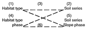
| (1) Habitat type |
(2) Soil series phase |
(3) E.L.U. (H.T. × S.S.) phase |
(4) Habitat type phase |
(5) Soil series slope phase |
(6) E.L.U. (H.T.P. × S.S.P.) |
|
|---|---|---|---|---|---|---|
| 1Mapping unit complexes of two or more series were included within series of the first name of the complex for this tabulation. | ||||||
| No. of types | 10 | 9 | 33 | 15 | 17 | 85 |
| No. of polygons | 62 | 33 | 109 | 103 | 52 | 199 |
| Average size polygons (acres) | 60 | 85 | 26 | 11 | 14 | 14 |
| Range in polygon sizes (acres) | 3 to 362 | 3 to 433 | 3 to 380 | 3 to 66 | 3 to 174 | 3 to 173 |
| Total forested acres | 2,804 | 2,804 | 2,804 | 2,804 | 2,804 | 2,804 |
 ECOLOGICAL LAND UNITS |
||||||
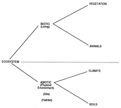
We are probably all on common ground with a general understanding of ecosystem concepts. We all have a holistic perspective. We understand that ecosystems are complex, multifactorial, interacting and interconnected, as well as varying in time and space. Changes are determined by many factors and difficult to predict with confidence. Our challenge over the years has been to describe, classify, and identify ecosystems to gain and communicate understanding of how they respond to management. One of the first steps is to illustrate the structure of ecosystems by separating and naming the components (fig. 2). Beyond this point is where most of us, through our education and experience, begin to diverge in perspectives.
Figure 2—Ecosystem structure. [Text description of this graph]
As soon as you focus on one of the components, the others become secondary. For example, all soil scientists are well grounded in Jenny's basic equation:
In a parallel fashion, plant ecologists are well grounded in Major's basic equation:
Each of these equations represents the concept of an integrated expression of the ecosystem. However, a common mistake is to let the similarity in the functional form of these equations suggest that plant ecologists and soil scientists should be in complete agreement—or that soils and vegetation should be closely correlated.
As individuals we each see the ecosystem from one point of view—our own. If we do not communicate well it is not because one point of view is wrong and another is right. It is only because our perspectives are different. When developing plans for a building, the architect must present several perspectives before a whole picture evolves. To have meaningful dialog, we must make the attempt to see the situation from more than a single perspective. Before we can develop a shared perspective, we must understand each other's perspectives. The following perspectives outline how we think a soil scientist and a vegetation specialist view an ecosystem, and suggests an ecological perspective that would serve both better.
If my focus begins with the soil, I am interested in what kinds of soils exist on the landscape (taxonomy), how they are distributed (mapping), and why they are different. What is the relative magnitude of each determining factor? Can I sort them out one at a time and then put them together? What is the relationship of a specific soil to each of the soil forming factors? I would guess that par-ent material and climate are dominant and expect that differences among soils become greater with time. Animal and vegetation effects are often secondary. Soil taxonomy is based primarily on morphology, although climatic effects are specifically incorporated at the third and fourth taxonomic levels for moisture and temperature regimes.
Once I feel comfortable with understanding the soil, then I can begin looking at relationships with the vegetation and potential vegetation. Relationships of soils to landforms and certain vegetation types are useful aids for mapping. A better understanding of soil-vegetation relationships would be very useful.
If my focus begins with the vegetation, I am interested in what kinds of plant communities exist on the landscape (taxonomy), how they are distributed (mapping), and why they are different. What is the relative magnitude of each determining factor? Can I sort them out one at a time and then put them together? What is the relationship of a specific plant community to each of the vegetation development factors? Parent material and climate are usually dominant factors and changes with time and disturbance are dramatic. Animals and soil variables (especially parent material and hydric soils) are important in many areas but are usually secondary. Vegetation taxonomy is based primarily on flora composition and structure. If variation in time can be sorted out by identifying potential natural vegetation types, then these associations can be used as an integrated expression of the physical environment commonly called a habitat type.
Once I feel comfortable with understanding the vegetation, then I can begin looking at relationships with the soils and topography. Topographic and parent material relationships are very helpful for mapping the habitat types. A better understanding of soil-vegetation relationships would be very useful.
This perspective is needed by soil scientists to help move toward being soil ecologists, as well as by vegetation specialists, so they may operate as plant ecologists. The ecosystem perspective is available for all specialists if they choose to think from that perspective, and if their education and philosophy allow. Are you satisfied with being soil scientists or would you rather be soil ecologists? Most of us have had some training in botany, soils, and ecology, but none has sufficient breadth and depth to be the ultimate expert in all three areas. We suggest that a sharing of talents and perspectives may provide the best hope for helping each other understand ecosystems and how to manage them.
The interrelationships of soil and vegetation have been a fascinating and frustrating area of investigation for many generations. Soil scientists and plant scientists have both championed their narrow, biased perspectives generally from the point of view that "my perspective is better than yours." We are all limited by our perspectives, or in current terminology, our paradigms. We all have a natural degree of "paradigm paralysis," blinding us to new ideas and different perspectives. Fortunately, there are some "paradigm pioneers" willing to risk ridicule by examining and trying new ideas.
One of us remembers well an incident where John Arnold, a landtype mapping pioneer at the Boise National Forest, and Bob Pfister, a young habitat type enthusiast, were making separate presentations during a Forest Service Educators Tour in the Payette National Forest in 1970. After each waxed eloquent on the value of these independent approaches to land management planning, old John took the young upstart aside over a bottle of Jack Daniels and said, "If we don't point out to all these administrators that both of our approaches have unique and complementary value, the chiefs will say, `Why do we need two approaches?' and will proceed to support one and throw the other one out." The next day we made a joint presentation, and the next week we were cooperating on a resource inventory of the Idaho Primitive Area. We did not call it that, but, in effect, we were working together to gain a shared ecosystem perspective.
The Society for Range Management has been actively debating soil-vegetation relationships and terminology during the 1980's. Although many individuals still do not agree, the framework is being laid for effective communication. The range site/habitat-type arguments may not be resolved until there is a one-generation turnover, but students of the subject will be approaching the subject with a broader paradigm than their predecessors. The principle of factor interaction and compensation makes it impossible for a habitat type to equal a range site if the former is based primarily on similar vegetation potential and the latter is based primarily on similar physical site characteristics. As John Arnold used to frequently remind people, "Wishing won't make it happen and saying it doesn't make it so."
Although many individuals have worked and are working hard to develop and demonstrate holistic perspectives for ecosystem classification and mapping, the universal solution has not yet been established. However, some benchmarks can be noted toward this end.
One example of a Forest Service mapping program was the Landtype Inventory in the Intermountain and Northern Regions during the 1970's (Wertz and Arnold 1972). These maps were based primarily on recognition of similar landform descriptions of major soils and habitat types as the source of management interpretations. They were especially useful for the ecological approach to land use planning that characterized the 1970's planning efforts. These maps probably should be dusted off and used as a layer in your developing Geographic Information Systems to help address current concerns dealing with landscape ecology.
In 1970 the Forest Service commissioned a task force to develop a single, hierarchical classification of ecosystems from existing information. The task force realized that responding fully to such a request was impossible, but suggested a methodology to meet the expressed objectives (Pfister and others 1972). This was approached from a mapping perspective where habitat type mapping and landtype mapping could be combined at different levels in their respective hierarchies to define an Ecological Land Unit, an area of land with defined similar vegetation potential and soil/landform characteristics. This attempt to reach an integrated ecosystem perspective was used by several people for planning in the 1970's with some modifications. The landtype mapping experts were reluctant to support the concept because they thought their landtype approach already did this. However, independent maps of landtype and landtype phase compared with habitat type maps suggested that theory and reality were not necessarily the same.
A decade later another task force focused on the taxonomy used to classify inventory points and provided the term Ecological Response Unit for any level of integration from potential vegetation types and soil taxonomy hierarchies (Driscoll and others 1984). The focus in this effort was on standardization of taxonomy for point identification. This provided a means to aggregate, but the link to mapping for disaggregation was not clearly established. In spite of five agencies approving the standardization, acceptance and use have not been automatic.
A Range Standardization Committee in the Society for Range Management has made good progress improving concepts and terminology. One or two major problems remain, but the desire and dedication are commendable. New terms have been defined to resolve ambiguities of older terms, but this does not necessarily solve the basic problems. A few of the definitions in the Society for Range Management (1989) glossary still represent unique perspectives within the profession.
The California National Forest System (Allen 1987) provides a good starting point for a regional program developed in the middle of widely varying viewpoints. The ecological type is basically a subdivision of a habitat type, where needed to reflect meaningful differences in soils or productivity within a habitat type.
We are probably all in complete conceptual agreement at the lowest level in any of these classifications. We could stand on the ground and agree on the smallest area that has similar vegetation potential, soils, and topography, and hence (we would hope) similar productivity potentials, hazards, and responses for management.
However, if classifications are useful only because they simplify to a number of categories that we can work with, then the ultimate question becomes one of scale and practicality. Within a State we would expect to have 30 to 80 forest habitat types and a similar number of soil series on forested lands. However, at the same level of ecological response units, ecological sites, or ecological types, as currently defined, we would expect 100 to 300 taxonomic units.
An alternative to taxonomy or mapping to the nth degree is to use multiple classifications that already exist to create unique units as needed. The National Land Classification experience offers the Ecological Response Unit concept for sorting, aggregating, and analyzing inventory and other data bases. The ECOCLASS experience offers the Ecological Land Unit concept for mapping, landscape ecology, and management. With the advent of GIS, this will be straightforward, objective, rapid, and efficient. Decisions must be based on appropriate levels of implementation (scale and costs) relative to objectives.
These ecosystem classification examples illustrate the difficulty of dealing with problems that are larger than a single profession. One approach is to try to expand the profession to cover the scope of the problem. However, the more logical approach may be for the professions to pool their collective expertise in teamwork endeavors for certain problems. The natural resource ecological issues of the 1990's will require a higher level of mutual support among agencies and professionals than ever before to maintain or regain leadership roles. This will require setting aside professional arrogance, agency arrogance, and the NIH (not invented here) syndrome. All we have is each other and a professional responsibility to manage natural resources for a sustainable society.
Allen, B. H. 1987. Ecological type classification for California: the Forest Service approach. Gen. Tech. Rep. PSW-98. Berkeley, CA: U.S. Department of Agriculture, Forest Service, Pacific Southwest Forest Range Experiment Station. 8p.
Arno, S. F. 1979. Forest regions of Montana. Res. Pap. INT-218. Ogden, UT: U.S. Department of Agriculture, Forest Service, Intermountain Forest and Range Experiment Station. 38 p.
Bailey, R. G. 1980. Description of the ecoregions of the United States. Misc. Publ. 1391. Washington, DC: U.S. Department of Agriculture, Forest Service. 77 p. Plus map.
Bassett, R.; Larson, M.; Moir, W. 1987. Forest and woodland habitat types (plant associations) of Arizona south of the Mogollon Rim and southwestern New Mexico. 2d ed. Albuquerque, NM: U.S. Department of Agriculture, Forest Service, Southwestern Region. 168 p.
Bradley, R. S. 1976. Precipitation history of the Rocky Mountain States. Boulder, CO: Westview Press. 334 p.
Daniels, J. D. 1969. Variation and intergradation in the grand fir-white fir complex. Moscow, ID: University of Idaho. 235 p. Dissertation.
Daubenmire, R. F. 1969. Structure and ecology of coniferous forests of the northern Rocky Mountains. In: Taber, R., ed. Coniferous forests of the northern Rocky Mountains: Symposium proceedings; 1968 September 17-20. Missoula, MT: University of Montana: 25-41.
Daubenmire, R. 1978. Plant geography. New York: Academic Press. 338 p.
Despain, D. G. 1973. Vegetation of the Big Horn Mountains, Wyoming, in relation to substrate and climate. Ecological Monographs. 43: 329-355.
DeVelice, R. L.; Ludwig, J. A.; Moir, W. H.; Ronco, F., Jr. 1986. A classification of forest habitat types of northern New Mexico and southern Colorado. Gen. Tech. Rep. RM-131. Fort Collins, CO: U.S. Department of Agriculture, Forest Service, Rocky Mountain Forest and Range Experiment Station. 59 p.
Driscoll, R. W.; Minkel, D. L.; Radloff, D. L.; Snyder, D. E.; Hagihara, J. S. 1984. An ecological land classification framework for the United States. Misc. Pub. 1439. Washington, DC: U.S. Department of Agriculture, Forest Service. 56 p.
Franklin, J. F.; Dyrness, C. T. 1973. Natural vegetation of Washington and Oregon. Gen. Tech. Rep. PNW-8. Portland, OR: U.S. Department of Agriculture, Forest Service, Pacific Northwest Forest and Range Experiment Station. 417 p.
Goldin, A.; Nimlos, T. J. 1977. Vegetation patterns on limestone and acid parent materials in the Garnet Mountains of western Montana. Northwest Science. 51(3): 149-160.
Hanks, J. P.; Fitzhugh, E. L.; Hanks, S. R. 1983. A habitat type classification system for ponderosa pine forests of northern Arizona. Gen. Tech. Rep. RM-97. Fort Collins, CO: U.S. Department of Agriculture, Forest Service, Rocky Mountain Forest and Range Experiment Station. 22 p.
Hoffman, G. R.; Alexander, R. R. 1976. Forest vegetation of the Bighorn Mountains, Wyoming: A habitat type classification. Res. Pap. RM-170. Fort Collins, CO: U.S. Department of Agriculture, Forest Service, Rocky Mountain Forest and Range Experiment Station. 38 p.
Layser, E. F.; Schubert, G. H. 1979. Preliminary classification for the coniferous forest and woodland series of Arizona and New Mexico. Res. Pap. RM-208. Fort Collins, CO: U.S. Department of Agriculture, Forest Service, Rocky Mountain Forest and Range Experiment Station. 27 p.
Marchand, D. E. 1973. Edaphic control of plant distribution in the White Mountains, eastern California. Ecology. 54: 233-250.
Moir, W. H.; Ludwig, J. A. 1979. A classification of spruce-fir and mixed conifer habitat types of Arizona and New Mexico. Res. Pap. RM-207. Fort Collins, CO: U.S. Department of Agriculture, Forest Service, Rocky Mountain Forest and Range Experiment Station. 47 p.
Neiman, K. E., Jr. 1986. Soil discriminant functions for six habitat types in northern Idaho. Moscow, ID: University of Idaho. 174 p. Dissertation.
Nimlos, T. J. 1986. Soils of Lubrecht Experimental Forest. Misc. Publ. 44. Missoula, MT: Montana Forest and Conservation Experiment Station, School of Forestry, University of Montana. 36 p. Plus appendixes.
Pfister, R. D. 1972. Vegetation and soils in the subalpine forests of Utah. Pullman, WA: Washington State University. 98 p. Dissertation.
Pfister, R. D.; Corliss, J. C.; [and others]. 1972. Ecoclass: a method for classifying ecosystemsa task force report to the Chief of the Forest Service. Ogden, UT: U.S. Department of Agriculture, Forest Service, Intermountain Forest and Range Experiment Station. 52 p.
Pfister, R. D.; Kovalchik, B. L.; Arno, S. F.; Presby, R. C. 1977. Forest habitat types of Montana. Gen. Tech. Rep. INT-34. Ogden, UT: U.S. Department of Agriculture, Forest Service, Intermountain Forest and Range Experiment Station. 174 p.
Rehfeldt, G. E. 1989. Ecological adaptations in Douglas-fir (Pseudotsuga menziesii var. glauca): a synthesis. Forest Ecology and Management. 28: 203-215.
Society for Range Management. 1989. A glossary of terms used in range management. 3d ed. Denver, CO: Society for Range Management. 20 p.
Soil Survey Staff. 1975. Soil taxonomy. Agric. Handb. 436. Washington, DC: U.S. Department of Agriculture, Soil Conservation Service. 753 p.
Steele, R.; Pfister, R. D.; Ryker, R. A.; Kittams, J. A. 1981. Forest habitat types of central Idaho. Gen. Tech. Rep. INT-114. Ogden, UT: U.S. Department of Agriculture, Forest Service, Intermountain Forest and Range Experiment Station. 138 p.
Steele, R. 1988. Ecological relationships of ponderosa pine. In: Baumgartner, D. M.; Lotan, J. E., eds. Ponderosa pine: the species and its management. Proceedings of the symposium; 1987 September 29-October 1. Spokane, WA: Washington State University, Cooperative Extension: 71-76.
Wellner, C. A. 1989. Classification of habitat types in the western United States. In: Ferguson, D. E.; Morgan, P.; Johnson, F. D., compilers. Proceedingsland classification based on vegetation: applications for resource management; 1987 November 17-19. Moscow, ID. Gen. Tech. Rep. INT-257. Ogden, UT: U.S. Department of Agriculture, Forest Service, Intermountain Research Station. 315 p.
Wertz, W. A.; Arnold, J. F. 1972. Land systems inventory. Ogden, UT: U.S. Department of Agriculture, Forest Service, Intermountain Region. 12 p.
Youngblood, A. P.; Mauk, R. L. 1985. Coniferous forest habitat types of central and southern Utah. Gen. Tech. Rep. INT-187. Ogden, UT: U.S. Department of Agriculture, Forest Service, Intermountain Forest and Range Experiment Station. 89 p.
Speakers answered questions from the audience after their presentations. Following are the questions and answers on this topic:
Q. With soil/vegetation interactions most prominent at forest-grassland interfaces, would the soil/vegetation interactions also be prominent at the geographical limits (particularly dry end) of individual species of conifers or understory vegetation?
A. Yes, species are often restricted to certain substrates near their dry geographical limits. This is particularly evident in the Wind River and Bighorn Ranges of Wyoming where many northern Rocky Mountain species are near their eastern limits at those latitudes.
Paper presented at the Symposium on Management and Productivity of Western-Montane Forest Soils, Boise, ID, April 10-12, 1990.
Robert Steele is Research Forester, Intermountain Research Station, Forest Service, U.S. Department of Agriculture, Boise, ID 83702; Robert D. Pfister is Research Professor, School of Forestry, University of Montana, Missoula, MT 59807.