LiDAR study – Multiscale Curvature Classification
LiDAR Classification
Multiscale Curvature Classification (Evans and Hudak 2007) is an iterative, multiscale approach for identifying positive curvatures representing non-ground returns in discrete return LiDAR. This old version of MCC software works on ArcInfo point coverages, is written in Arc Macro Language, and is slow. We recommend using the current MCC-LIDAR software hosted on SourceForge (https://sourceforge.net/apps/trac/mcclidar/), which reads/writes lidar .las format files, is written in c++, and is fast.
For information regarding this algorithm please contact
Andrew T. Hudak - Research Forester / Landscape Ecologist
USFS – Rocky Mt. Research Station, Forestry Sciences Lab
1221 South Main St.
Moscow, Idaho, 83843
ahudak[at]fs.fed.us
A large portion of LiDAR acquisition cost is incurred during post-processing to separate ground from non-ground returns.
This is in large part due to the manual editing required to "clean up" the surface and the need to reclaim software
development or purchase costs.
LiDAR vendors have put forth substantial investment into development of ground identification algorithms.
Unfortunately, the majority of available algorithms are proprietary and available only in commercial software or through
"in-house" vendor processing at considerable cost.
Ground information is often delivered in the form of gridded raster or normally spaced point data.
Both of these deliverables generalize the data, discarding the original spatial precision and volume of ground returns.
The original volume of ground returns is needed to build relationships between ground and vegetation returns.
If an appropriate volume of ground returns is retained, then the resulting interpolated surface will match the scale
and precision of the original LiDAR point cloud, reducing bias and error in the derived heights.
A simple differencing of the interpolated ground height surface from the raw LiDAR elevations will provide
the vegetation height at each point while preserving density relationships related to vegetation cover,
such as the proportion of non-ground to ground returns.
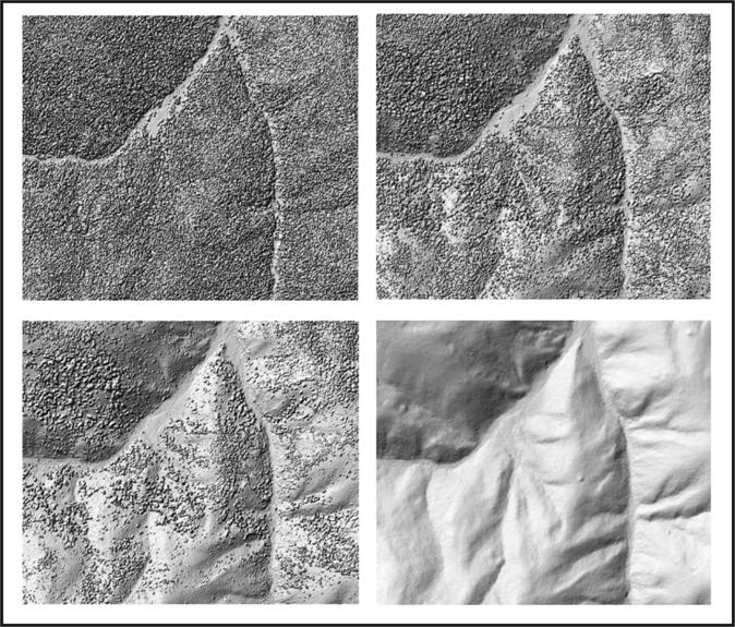
Example of MCC model in high biomass forest in northern Idaho across 3 model loops.
References:
J.S. Evans, A.T. Hudak. 2007. A Multiscale Curvature Algorithm for Classifying Discrete Return LiDAR in Forested Environments. IEEE Transactions on Geoscience and Remote Sensing 45:4 pp.1029-1038.
R.A. Haugerud, D.J. Harding. 2001. Some Algorithms for Virtual Deforestation (VDF) of Lidar Topographic Survey Data. International Archives of Photogrammetry and Remote Sensing, Graz, Austria, vol. XXXIV-3/W4, pp. 211-217.
Model Usage:
MCC <INCOVER> <OUTCOVER> <ELEVATION ITEM> <SCALE>
        {CURVATURE} {COLUMNS-X} {COLUMNS-Y}

INCOVER - Point coverage of LiDAR point cloud
OUTCOVER - Coverage of identified LiDAR ground returns
ELEVATION ITEM - Info item in LiDAR-coverage, containing elevation value
SCALE - Scale parameter
CURVATURE - Coefficient defining curvature threshold
COLUMNS-X - Number of divisions on X plane
COLUMNS-Y - Number of divisions on Y plane
The curvature coefficient for ~2 meter postspacing can be set to 0.2 - 0.3,
for < 1 meter postspacing depending on the density of the canopy
I have set it to 0.7.
This may require some trial and error to find the ideal starting value.
The scale and curvature coefficients are defined automatically in subsequent model loops,
thus requiring only a starting value.
The scale parameter is initially derived from the nominal postspacing.
The COLUMNS-X and COLUMNS-Y arguments are for an automatic tiling scheme within the model.
The tiling is corrected for edge effect and is meant to speed up processing and accommodate the limit of samples
the spline can fit (400,000 point max).
The best way to determine these arguments is to take the total number of points in a given coverage
and figure out the number of tiles you need to have <= 400,000 points per tile.
The AML merges the tiles so the final coverage is a new coverage containing the filtered ground returns.
The model assumes an unfiltered point cloud.
If the LiDAR data has already been filtered by the vendor or is gridded, MCC will not provide correct results.
A second version of the model has been implemented using the IFD (Iterative Finite Differencing) spline model.
This method is much faster and does not require a tiling scheme.
However, care must be taken in certain landscapes not to classify ground returns as positive curvatures.
In very steep terrains erosion of the hillslope has been observed.
This can often be addressed by changing the model parameters.
An additional parameter has been added to adjust the spline tension f which can mitigate
over-classification by altering the magnitude of the curvature.
The model is set up as an ATOOL.
If you put it in the $ARCHOME\atool\arc directory it will act like a native ArcInfo command.
An example of this path, depending on the version you are running, is:
C:\arcgis\arcexe9x\atool\arc
DOWNLOAD MCC
DOWNLOAD MCC_IFD